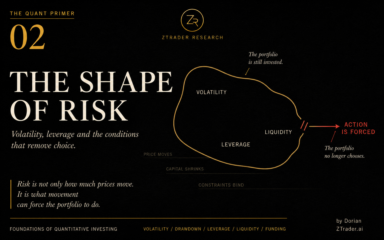
THE QUANT PRIMER 02 | THE SHAPE OF RISK

Volatility, leverage and the conditions that remove choice

Risk becomes easier to discuss after it has been compressed into a number.

In the quant world there are many metrics to compare: A portfolio runs at twelve percent volatility. The position contributes forty basis points of daily value-at-risk. The systematic fund targets a ten percent annualized standard deviation.

These figures are useful because they allow exposures with different prices, units and histories to enter a common risk budget. Once the calculation appears on a screen, however, description begins to masquerade as explanation.

Volatility measures the dispersion of returns. Capital encounters something more conditional.

A loss may arrive gradually in a deep market, leaving the investor free to reduce exposure. It may appear suddenly after months of apparent stability, just as liquidity retreats and financing terms tighten. The measured movement can be identical while the economic consequences differ because one portfolio retains control and the other does not.

That distinction defines the subject of this Primer.

Risk is not simply the possibility that prices move. It is the possibility that movement changes what the investor is able to do next.

1. What the number contains

Historical volatility estimates how widely observed returns varied around their mean during a selected period. The estimate depends on choices that are often hidden by the final decimal: sampling frequency, lookback window, weighting method and treatment of extreme observations.

None of this makes volatility arbitrary. It makes the number conditional.

A sixty-day estimate answers a different question from a five-year estimate. An exponentially weighted model reacts more quickly to recent events than an equally weighted sample. Daily data can conceal intraday instability, while high-frequency data introduces market-microstructure noise. The calculation is precise only after the researcher has decided which history should matter.

The same limitation follows volatility into portfolio construction. A common scaling rule sets exposure inversely to estimated risk:

w_t = k\frac{\sigma^*}{\widehat{\sigma}_t}

where \sigma^* is the target volatility, \widehat{\sigma}_t is the current estimate and k incorporates other portfolio constraints.

If estimated volatility falls, permitted exposure rises. If volatility doubles, exposure is cut roughly in half.

The rule is internally coherent, but it does not determine whether the low estimate represents durable stability or merely a quiet interval before the distribution changes.

Moreira and Muir found that portfolios reducing exposure when factor volatility was high produced substantially higher Sharpe ratios across several equity factors and currency carry in their sample. Their explanation was not that high volatility is always bearish.

Factor volatility varied far more than expected returns, so maintaining constant exposure during volatile periods often delivered poor compensation for the additional risk. (NBER⁠)

That result supports volatility management as a serious portfolio technique.

It does not turn recent calm into proof of safety.

2. Calm can become an input into leverage

A quiet market does more than reduce the number displayed beside “risk.” It changes the amount of exposure that institutions are permitted or willing to hold.

Lower realized volatility can expand risk budgets. Rising collateral values improve borrowing capacity. Narrower spreads make leveraged trades appear easier to finance and exit.

Each response is reasonable when viewed separately; together they can create a system whose apparent stability depends on leverage continuing to be available.

The process is procyclical. Market-sensitive valuations and leverage practices can encourage balance sheets to expand during favorable conditions and contract once prices and measured risk move against them. The Committee on the Global Financial System identified this interaction between valuation, leverage and funding liquidity as an important source of financial procyclicality.

No single investor needs to believe that low volatility eliminates risk. Similar constraints are enough.

One risk-parity fund adds exposure because covariance estimates have declined.

The other relative-value fund increases gross leverage because financing remains cheap.

The dealer permits larger positions because collateral is stable.

Even different mandates produce the same directional adjustment.

The market looks calm partly because participants have adapted their balance sheets to calm.

The vulnerability appears when the condition supporting those balance sheets changes.

3. Returns arrive in an order

A distribution treats returns as observations. A portfolio experiences them as a sequence.

Begin with two unlevered portfolios, each worth $100. Both experience one gain of 20 percent and one loss of 20 percent. Regardless of order, the terminal value is $96:

100 \times 1.20 \times 0.80 = 96

Compounding creates the four-dollar loss. Sequence alone does not.

Now introduce a constraint.

Portfolio A gains 20 percent first, reaching $120, then loses 20 percent and finishes at $96.

Portfolio B loses 20 percent first. Its lender responds by cutting the permitted exposure in half. The remaining capital participates in only half of the subsequent 20 percent recovery:

100 \times 0.80 \times 1.10 = 88

The underlying market returns are unchanged. The investor’s path is not.

A loss arriving early reduced the capital base and triggered a change in exposure before the recovery occurred. The portfolio was still capable of recovering in statistical terms, but the financing structure no longer allowed it to own the same position.

Drawdown begins to describe this problem more directly than variance because it measures the capital lost from a previous peak.

Duration adds another dimension. A sharp decline followed by rapid recovery imposes a different burden from an equally deep drawdown that traps capital below its high-water mark for years.

Neither metric predicts the future. Together they reveal something volatility suppresses: losses have a location in time, and that location can alter the strategy itself.

4. The real risk limit is forced action

Investors often describe risk tolerance as though survival depended only on temperament.

A fund may claim it can tolerate a twenty percent drawdown. That statement is irrelevant if redemptions begin at ten percent, a prime broker changes margin terms at twelve or a mandate requires exposure to be reduced at fifteen. The loss an investor is willing to accept and the loss the structure can absorb are different quantities.

The second one matters more.

Capacity is determined by collateral, funding, liabilities, redemption terms, regulatory capital and the behavior of counterparties. These constraints can convert an unfavorable price move into mandatory action.

Once the portfolio must sell, risk is no longer a forecast about where the asset eventually trades. It becomes a question of what price the balance sheet can survive today.

Leverage makes this transition nonlinear. Borrowing magnifies the initial asset loss, but the next stage matters more: lower equity supports less borrowing, higher volatility invites larger haircuts, and reduced financing forces the portfolio to sell into the same market that weakened its collateral.

The relevant distance is not between today’s price and an arbitrary stop.

It is between current conditions and the first constraint capable of removing discretion.

CHART 01 — SAME VOLATILITY, DIFFERENT SURVIVAL

5. Liquidity belongs inside the position

A portfolio is marked using current prices. Risk calculations then tend to assume that exposure could be changed somewhere near those marks.

That assumption is most comfortable before anyone needs to test it.

Market liquidity concerns the ability to trade without moving the price excessively. Funding liquidity concerns the ability to obtain or retain the financing needed to hold the position. Brunnermeier and Pedersen showed how the two can reinforce each other: deteriorating market liquidity raises funding pressure, while constrained funding reduces traders’ ability to provide market liquidity. Under certain conditions, higher margins amplify rather than absorb the shock. (NBER⁠)

A stop-loss does not solve this problem. It identifies a price at which the strategy would prefer to exit, not the price available after many holders reach the same conclusion.

During stress, the intended exit may become a market order competing with every other balance sheet trying to conserve cash.

March 2020 provided a concrete example. Leveraged relative-value investors in US Treasury markets faced margin and funding pressure as normally small pricing relationships moved sharply. Forced sales and constrained dealer intermediation contributed to dysfunction in a market usually treated as one of the world’s deepest.

Liquidity is not a permanent property stored inside an asset.

It is a service supplied by other balance sheets, often under terms that change precisely when the portfolio needs the service most.

6. Correlation can become a funding relationship

Diversification depends on positions responding differently to the forces that determine returns. Historical covariance is the standard way to estimate those relationships, and under ordinary conditions it can be highly informative.

Stress introduces a different organizing principle.

An equity index, a currency carry trade and a credit position may have distinct economic exposures, but they can still be owned by investors using the same financing channels. Once those investors need cash, the common factor is no longer growth, inflation or valuation. It is liquidation.

Assets that looked separate by instrument become connected through ownership, collateral and the need to reduce gross exposure.

Currency carry illustrates the mechanism. Brunnermeier, Nagel and Pedersen documented negative skew in carry-trade returns and linked crashes to sudden unwinds during periods of deteriorating risk appetite and funding liquidity. (NBER⁠)

A correlation matrix estimated in calm markets may therefore miss the relationship that dominates during forced deleveraging. The statistical diversification was real within the sample.

The financing concentration existed outside the matrix.

Diversification should be evaluated twice:

first by return behavior;

then by the mechanisms capable of forcing positions through the same exit.

7. Smooth returns may be deferred liabilities

Some strategies earn a premium by accepting losses that arrive infrequently.

Insurance produces a recognizable version of this profile. Premium income is steady; claims are irregular. The absence of a claim during a given month does not mean the insurer generated free alpha. It means the liability did not mature during that interval.

Financial markets contain equivalent structures.

Short-volatility strategies receive option premium while retaining exposure to discontinuous movement.

Credit earns spread while bearing default and liquidity risk. Carry strategies collect yield differentials while remaining vulnerable to funding shocks and crowded unwinds.

Relative-value trades harvest small price discrepancies while relying on convergence, leverage and continued financing.

These returns can look unusually efficient during ordinary periods because the premium is recorded continuously while the associated loss is episodic. High hit rates and low recent volatility then become mistaken for evidence that the exposure is inherently safe.

The correct question is not whether the strategy has produced stable returns.

It is what obligation those returns have been financing.

Negative skew is not automatically a defect. An investor may rationally accept tail exposure at the right price.

The analytical failure occurs when compensation for bearing a known liability is relabeled as unexplained alpha.

8. Risk control has an execution price

A volatility-targeting rule is designed to reduce exposure when estimated risk rises.

On paper, the adjustment is immediate and clean.

Markets charge for the transition.

Suppose a portfolio targets ten percent volatility. Its estimate rises from ten to twenty percent. All else equal, the permitted exposure falls by half. The strategy has not formed a bearish view. Its position is now too large for the mandate.

If the market remains liquid, the adjustment may work as intended.

Under stress, spreads widen, market depth falls and other investors may be responding to similar constraints. Reducing modeled risk then requires buying scarce liquidity at an unfavorable moment.

The episode need not be caused by volatility-targeting funds for the mechanism to matter. March 2020 showed the broader structure clearly: rising volatility, margin calls, leverage reduction and intermediation bottlenecks interacted across Treasury and funding markets.

This distinction matters because volatility control is sometimes criticized too casually. The rule can improve portfolio behavior over time, as Moreira and Muir’s empirical results suggest. The vulnerability lies in pretending that the required position change can always be executed at the price embedded in the model. (NBER⁠)

Risk reduction is a trade.

It has timing, capacity and market impact like every other one.

CHART 02 — WHEN CALM BECOMES LEVERAGE

9. Models fail at their boundaries

Unexpected losses are often followed by proposals to refine the distribution: use fatter tails, shorten the volatility window, raise the confidence level or make correlations more responsive.

Those changes may improve the estimate. They do not address every failure.

A model can calculate precisely while its operating assumptions deteriorate. The quoted spread may not support the desired order size. Financing may no longer be available on historical terms. Several hedges may depend on the same dealer capacity. A correlation estimate may describe normal economic relationships while the portfolio has entered a common liquidation event.

Increasing value-at-risk from a 95 to a 99 percent confidence level does not solve a discontinuous market, uncertain financing or an exit shared with crowded positions. The additional decimal creates statistical conservatism without necessarily adding structural realism.

Every risk estimate should therefore be read as a conditional statement:

Given these assumptions about returns, liquidity, financing and behavior, the portfolio is expected to lose no more than this amount with the stated frequency.

Risk management begins by identifying which assumptions carry the most weight and what happens when several fail together.

The formula measures the portfolio inside a structure.

The risk lies partly in the structure itself.

10. A portfolio needs several risk languages

No single statistic can answer every question because portfolio failure has more than one mechanism.

Volatility estimates the ordinary scale of variation.

Drawdown records capital lost from a previous peak.

Skew describes asymmetry.

Tail measures examine extreme regions of the distribution.

Leverage determines how asset losses transmit into equity.

Liquidity analysis estimates the time and concession required to change exposure.

Stress tests examine specified shocks, including combinations not present in the historical sample.

Concentration analysis identifies positions that appear diverse but depend on the same economic thesis, financing source or exit route.

The objective is not to accumulate metrics until the dashboard resembles an aircraft cockpit designed by a committee. More numbers can hide the absence of a coherent diagnosis just as easily as one number can.

A useful risk process should answer four questions plainly:

1. What causes the portfolio to lose?

2. What makes that loss accelerate?

3. Which constraint could force action?

4. What remains tradable when action becomes necessary?

Volatility contributes to each answer.

It is not the answer itself.

CHART 03 — THE CONDITIONS OF SURVIVAL

Conclusion

Volatility remains indispensable because it gives heterogeneous positions a common unit. It helps scale exposure, combine assets and impose discipline on portfolios that would otherwise rely on intuition.

Its convenience becomes dangerous only when the unit replaces the mechanism.

Portfolios do not fail because a standard deviation crossed an abstract threshold. They fail when price movement meets leverage, when collateral terms change, when several positions depend on the same liquidity, or when an investor expected to be patient discovers that someone else controls the timetable.

The critical distinction is not between calm and volatile markets.

It is between a portfolio that still has choices and one whose next action has already been dictated.

Research References:

1. Moreira, Alan; Muir, Tyler. Volatility-Managed Portfolios. NBER Working Paper No. 22208; subsequently published in The Journal of Finance. (NBER⁠)

2. Brunnermeier, Markus K.; Pedersen, Lasse Heje. Market Liquidity and Funding Liquidity. NBER Working Paper No. 12939; subsequently published in The Review of Financial Studies. (NBER⁠)

3. Brunnermeier, Markus K.; Nagel, Stefan; Pedersen, Lasse Heje. Carry Trades and Currency Crashes. NBER Working Paper No. 14473. (NBER⁠)

4. Committee on the Global Financial System. The Role of Valuation and Leverage in Procyclicality. CGFS Papers No. 34, Bank for International Settlements. (BIS⁠)

5. Schrimpf, Andreas; Shin, Hyun Song; Sushko, Vladyslav. Leverage and Margin Spirals in Fixed Income Markets During the Covid-19 Crisis. BIS Bulletin No. 2. (BIS⁠)

6. Avalos, Fernando; Ehlers, Torsten; Eren, Egemen. BIS analysis of margin leverage and vulnerabilities in US Treasury futures. (BIS⁠)